Data preparation
After completing the delineation of the watershed and the associated hydrological response units (HRUs), we have come to the point of selecting and preparing the available meteorological data. With this data, we will be able to (1) define the long-term climate within the watershed and (2) use actual time series of meteorological conditions in specific locations that will steer the hydrological behaviour of the watershed. Keeping this in mind, our first step is determining what kind of data we actually need and where we can find it, followed by bringing all this data together and cleaning it up to a level that is acceptable for our project. While this sounds simple, it will easily take up most of the time, so let's get started!
We start with identifying the necessary data. While SWAT+ actually does not need any external data to develop a hydrological model, it is desirable to have some flow data available for model calibration. This type of data is typically derived from water level readings and point-specific discharge curves that link overall flow with the water level. Ideally, this flow data has a daily resolution that can additionally be used to derive monthly conditions. For the Paute watershed, we collected several time series of (derived) river flow for a variety of stations throughout the basin from INAMHI, ETAPA, and CELEC.
In addition to (daily) flow data, precipitation data greatly contributes to the calibration of the hydrological model as it is one of the main steering factors of river flow. Even more so, also relative humidity, air temperature, wind speed, and solar radiation play a role in the associated relevant (atmospheric) processes. As a result, we prefer to have (daily) time series of these variables available to accurately simulate the meteorological conditions within the basin. For the Paute watershed, we collected several time series of all five meteorological variables for a variety of stations throughout the basin from INAMHI and ETAPA. But, these data sets are also characterized by high levels of missing data...
Data sources
Overlapping stations
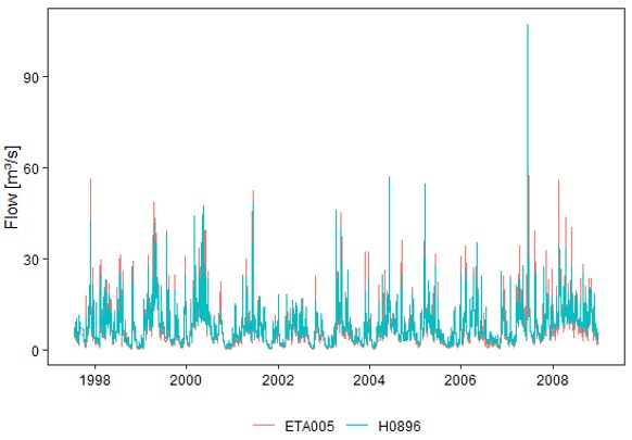 We start our assessment with a geographical analysis and the identification
of overlapping stations. These are stations that are situated in the same river or located within a couple of kilometers from one another. By identifying these
stations and comparing their time series, we can confirm their reliability or flag them for further review later on. The graph on the right illustrates such a
comparison for two hydrological stations in Sayausi, indicating very similar patterns.
We start our assessment with a geographical analysis and the identification
of overlapping stations. These are stations that are situated in the same river or located within a couple of kilometers from one another. By identifying these
stations and comparing their time series, we can confirm their reliability or flag them for further review later on. The graph on the right illustrates such a
comparison for two hydrological stations in Sayausi, indicating very similar patterns.
Stations without coordinates
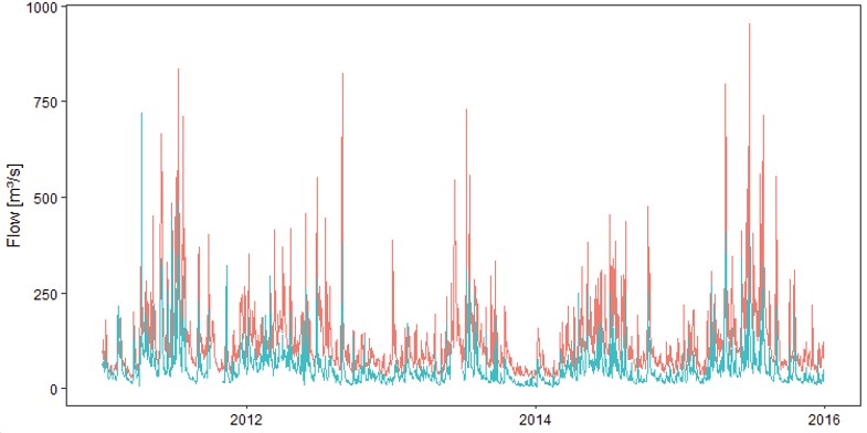 While overlapping stations can confirm time series and recorded environmental
conditions, there are time series for which it is unclear where exactly the data originates from (i.e., where the associated station should be located). One of
the examples is the data that can be downloaded here. From this site,
information can be obtained on the flow of the Paute river (since 2010) and the flows of the different generators (Mazar (since 2010), Amaluza (since 1985), and
Sopladora (since 2016)). However, it is unclear how these relate to other hydrological stations within the watershed. The graph on the right illustrates the
difference in flow between the INAMHI station in Paute (blue) and the time series from the webpage (red).
While overlapping stations can confirm time series and recorded environmental
conditions, there are time series for which it is unclear where exactly the data originates from (i.e., where the associated station should be located). One of
the examples is the data that can be downloaded here. From this site,
information can be obtained on the flow of the Paute river (since 2010) and the flows of the different generators (Mazar (since 2010), Amaluza (since 1985), and
Sopladora (since 2016)). However, it is unclear how these relate to other hydrological stations within the watershed. The graph on the right illustrates the
difference in flow between the INAMHI station in Paute (blue) and the time series from the webpage (red).
Flow data
Data selection
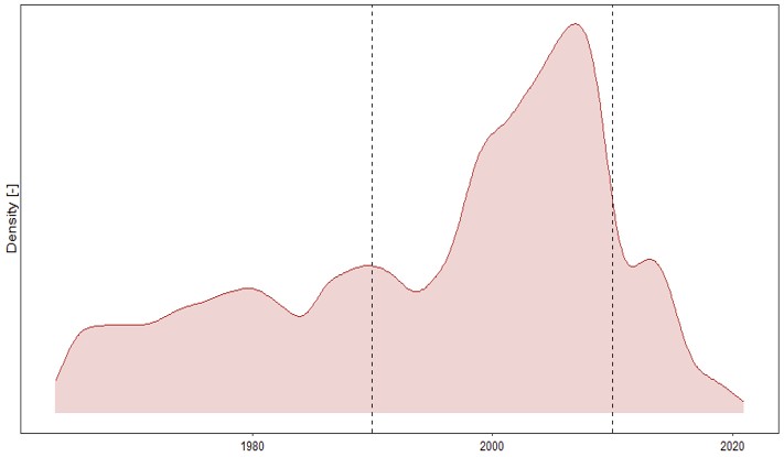 We start the selection of flow data with an arbitrary statement on the
desired number of data points. In this case, we keep only those stations with 5 years of data (or about 1825 daily data points). Then, we assess the temporal
distribution of these data points to determine which period in time is characterized by the most data points. While mostly visual, this approach relies on the idea
that the period in time with the most data points will also allow a stronger calibration and validation of the hydrological model. After identifying this moment,
a sufficiently long period is chosen for both calibration (e.g. 15 years) and validation (e.g., 5 years). The graph on the right illustrates this approach and also
identifies the period from 1990 up to 2010 as ideal for model calibration and validation.
We start the selection of flow data with an arbitrary statement on the
desired number of data points. In this case, we keep only those stations with 5 years of data (or about 1825 daily data points). Then, we assess the temporal
distribution of these data points to determine which period in time is characterized by the most data points. While mostly visual, this approach relies on the idea
that the period in time with the most data points will also allow a stronger calibration and validation of the hydrological model. After identifying this moment,
a sufficiently long period is chosen for both calibration (e.g. 15 years) and validation (e.g., 5 years). The graph on the right illustrates this approach and also
identifies the period from 1990 up to 2010 as ideal for model calibration and validation.
Data cleaning
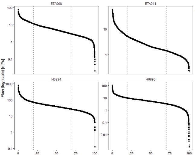 The previous section describes the flow data as it is available and prior to
any cleaning. As it is possible that not all values are correct or plausible, we are going to assess the data quality. To do so, we will apply a within-station and
between-station approach. We start with depicting the flow duration curves to help us with detecting potential irregularities at the outer ends and define logical
values for the minimum and maximum flows within each station. An illustration of this type of graphs is provided on the right. Then, time series of stations within
the same subbasin are visualised to identify strange or sudden behaviour that contrasts strongly with the other stations in the same basin. It goes without saying
that the applied assessments and corrections in this step are highly arbitrary and open for discussion.
The previous section describes the flow data as it is available and prior to
any cleaning. As it is possible that not all values are correct or plausible, we are going to assess the data quality. To do so, we will apply a within-station and
between-station approach. We start with depicting the flow duration curves to help us with detecting potential irregularities at the outer ends and define logical
values for the minimum and maximum flows within each station. An illustration of this type of graphs is provided on the right. Then, time series of stations within
the same subbasin are visualised to identify strange or sudden behaviour that contrasts strongly with the other stations in the same basin. It goes without saying
that the applied assessments and corrections in this step are highly arbitrary and open for discussion.
Meteorological data
Weather generator
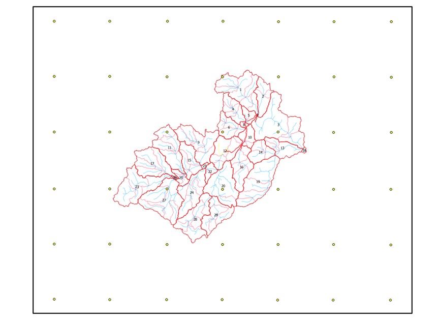 First of all, it is good to be aware that SWAT+ provides its own
weather generator to create climatic conditions and daily weather events. However, as this model has been developed for the contiguous United States, it is
strongly recommended to use observed data whenever possible (for more information on the Weather generator: check
here). For our watershed,
the generator creates a series of 42 climate stations throughout the basin, with some locations relatively far away from the study area.
First of all, it is good to be aware that SWAT+ provides its own
weather generator to create climatic conditions and daily weather events. However, as this model has been developed for the contiguous United States, it is
strongly recommended to use observed data whenever possible (for more information on the Weather generator: check
here). For our watershed,
the generator creates a series of 42 climate stations throughout the basin, with some locations relatively far away from the study area.
While this grid has been developed by the weather generator, we can replace it completely with our own weather stations. To do so, it is good to be aware of the information that we have to provide to each of these stations to support the functioning of the underlying climate model and the generation of realistic weather conditions throughout the basin. These are all the included meteorological parameters:
- Average daily maximum air temperature (°C)
- Average daily minimum air temperature (°C)
- Standard deviation for daily maximum air temperature (°C)
- Standard deviation for daily minimum air temperature (°C)
- Average total month precipitation (mm)
- Standard deviation of daily precipitation (mm/d)
- Skewness coefficient of daily rainfall within a month (mm)
- Probability of a wet day after (1) a wet day and (2) a dry day (-)
- Average number of precipitation days per month (-)
- Maximum half-hourly rainfall per month (mm)
- Average daily solar radiation (MJ/m²/d)
- Average daily dewpoint temperature (°C) OR average daily humidity (-)
- Average wind speed (m/s)
This overview also allows to identify which parameters can be updated based on observed data (ETAPA, INAMHI, …) and which ones require an alternative solution. This can include the use of climate data in the nearest station created by the weather generator, as well as the use of satellite data. Based on this list of 13 parameters, we can already conclude that the following parameters cannot be calculated with the available observed data:
- Statistics for temperature, as only daily averages are available
- Maximum half-hourly rainfall per month, as only daily totals are available
- Statistics for solar radiation, as only daily hours of sunshine are available
Weather data
Observed weather data works in cooperation with the weather generator to derive viable weather conditions throughout the basin. Various weather stations can be identified that have time series of a set of meteorological variables, in which data can be missing (though replaced by the value -99, which indicates that it has to be simulated) and a whole time series can be absent (a 'virtual' station to avoid selection of the closest weather station). More information on these empty data series will be provided later on. The cooperation with the weather generator relies on the inclusion of the following five variables:
- Precipitation (table 'pcp', includes the total daily rainfall in mm)
- Temperature (table 'tmp', includes minimum and maximum of the day in °C)
- Solar radiation (table 'slr', includes average radiation in MJ/m²/d)
- Humidity (table 'hmd', includes average daily humidity as a fraction)
- Wind (table 'wnd', includes average daily wind speed in m/s)
This overview also allows to identify which parameters can be updated based on observed data (ETAPA, INAMHI, …) and which ones require an alternative solution. This can include the use of climate data in the nearest station created by the weather generator, as well as the use of satellite data. Based on this list of 5 parameters, we can already conclude that the following parameters cannot be calculated with the available observed data:
- Temperature, as only daily averages are available
- Solar radiation, as only daily hours of sunshine are available
Observed data
Based on the assessment of the previous two sections, the following variables are selected for further analysis of the external data (ETAPA, INAMHI, …): (1) Precipitation, (2) Humidity, and (3) Wind speed. Similar to the external flow data, we start by retaining only those stations with at least 5 years of daily precipitation data within the calibration-validation period (01/01/1990-31/12/2009). These are the stations that we will be using for all meteorological variables (even when no observed data is available). After this selection of which stations to consider, we continue with subsetting the available time series to cover the time period 01/01/1980 up to 31/12/2009. This period covers a 10-year warming period for the SWAT+ model, a 15-year calibration period, and a 5-year validation period. Moreover, by covering 30 years of weather data, it provides a solid basis to derive month-specific weather statistics for the weather generator. We will tackle each considered variable in more detail in the following paragraphs.
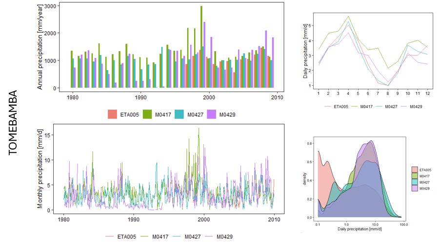 We start the more detailed assessment with the precipitation
data. Following the initial spatial and temporal filtering, we continue with an assessment of consistency. To do so, we look at inconsistencies in the
precipitation time series between stations that are located close to one another. This allows to (1) exclude stations with overall inconsistent patterns and
(2) to exclude specific periods in time for a specific station. The graph on the right illustrates this approach for the Tomebamba river, for which we have
four different meteorological stations with precipitation data. From this, a diverging station (M0429) and period (1997-1999) can be derived. Following this
general screening, more attention is given to the individual stations and potential extreme values. These detailed assessment can lead to the exclusion of
any extreme value from the meteorological basis.
We start the more detailed assessment with the precipitation
data. Following the initial spatial and temporal filtering, we continue with an assessment of consistency. To do so, we look at inconsistencies in the
precipitation time series between stations that are located close to one another. This allows to (1) exclude stations with overall inconsistent patterns and
(2) to exclude specific periods in time for a specific station. The graph on the right illustrates this approach for the Tomebamba river, for which we have
four different meteorological stations with precipitation data. From this, a diverging station (M0429) and period (1997-1999) can be derived. Following this
general screening, more attention is given to the individual stations and potential extreme values. These detailed assessment can lead to the exclusion of
any extreme value from the meteorological basis.
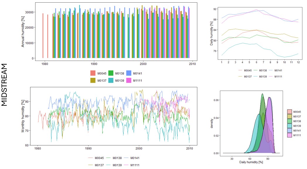 Whereas precipitation is characterised by an extensive set of viable
stations, this is not the case for humidity and wind speed. Nevertheless, we apply a similar approach as mentioned for precipitation. From this, we expect
no big differences between stations and a relatively unimodal behaviour (contrasting precipitation). The graph on the right illustrates this by looking into the
relative humidity data that we have available for the whole Paute basin, which are mostly located in the midstream area of the basin. From this, a high
degree of similarity in relative humidity can be assumed for the considered stations. Still, we rely on an additional assessment of potential extreme values
to further clean this data.
Whereas precipitation is characterised by an extensive set of viable
stations, this is not the case for humidity and wind speed. Nevertheless, we apply a similar approach as mentioned for precipitation. From this, we expect
no big differences between stations and a relatively unimodal behaviour (contrasting precipitation). The graph on the right illustrates this by looking into the
relative humidity data that we have available for the whole Paute basin, which are mostly located in the midstream area of the basin. From this, a high
degree of similarity in relative humidity can be assumed for the considered stations. Still, we rely on an additional assessment of potential extreme values
to further clean this data.
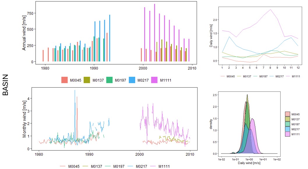 A similar assessment of the observed wind speed is expected to
indicate some larger differences between stations. The graph on the right illustrates this by looking into the wind speed data that we have available for the
whole Paute basin, which are located throughout the whole basin. From this, quite some variability in the observed wind speed can be derived, including
a diverging station (M1111) and period (1990-1994). Following this, a final assessment of potential extreme values is implemented to further clean the data and
avoid any large distortion of the derived monthly statistics.
A similar assessment of the observed wind speed is expected to
indicate some larger differences between stations. The graph on the right illustrates this by looking into the wind speed data that we have available for the
whole Paute basin, which are located throughout the whole basin. From this, quite some variability in the observed wind speed can be derived, including
a diverging station (M1111) and period (1990-1994). Following this, a final assessment of potential extreme values is implemented to further clean the data and
avoid any large distortion of the derived monthly statistics.
As time series of both relative humidity and wind speed display a limited spatial coverage, we are faced with the challenge to find monthly climate statistics for both variables in the stations withouth any observed time series. Here, we can opt to (1) copy the baseline weather generator monthly values for these variables from the closest station or (2) copy the monthly statistics of the closest field station. To support our decision, we can implement a comparison of the field data with the closest weather generator station. For now, we will use the closest field station to fill our database with monthly statistics (which also reduces our dependence on the built-in weather generator). The daily time series will remain empty, though.
Satellite data
Based on the assessment of the first two subsections, the following variables are selected for further analysis of the satellite data (CDS ERA5, starting from 1940): (1) Temperature and (2) Radiation. We will do this for all stations with sufficient precipitation data (see previous section).
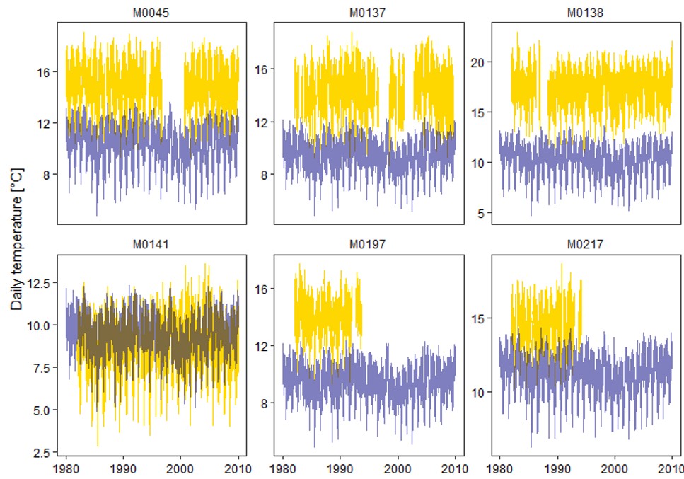 We start by directing our focus towards temperature and comparing
the observed daily temperature (provided by INAMHI and ETAPA) with the derived daily temperature from the Copernicus ERA5 Reanalysed Land Data set. Based on this
analysis, we implement a correction to align the remote data more accurately with field observations. To do so, we can (1) rely on the daily temperature ratios
to derive maximum and minimum daily temperatures from observations or (2) derive linear models that link observations with the satellite-based data. For the
project at hand, we will make use of the first approach. More specifically, daily maximum and minimum temperatures are derived from the hourly satellite-based
data and set out against the daily average to obtain a ratio (i.e. “X times higher/lower than the daily average”). These ratios are subsequently used to transform
the observed series of daily averages into series of daily maximum and minimum temperatures, by using station-and date-specific ratios. The graph on the right
illustrates this approach (yellow as the observed temperature and blue as the satellite-based temperature) and shows that a correction is clearly needed, though
dependent on the station. This approach allows to convert observed temperature time series and derive the necessary monthly statistics of stations with observed
data. For stations without any observations, the monthly statistics are copied from the closest station with observations and corrected for the difference in
altitude (at -6.5 °C per 1000 m increase).
We start by directing our focus towards temperature and comparing
the observed daily temperature (provided by INAMHI and ETAPA) with the derived daily temperature from the Copernicus ERA5 Reanalysed Land Data set. Based on this
analysis, we implement a correction to align the remote data more accurately with field observations. To do so, we can (1) rely on the daily temperature ratios
to derive maximum and minimum daily temperatures from observations or (2) derive linear models that link observations with the satellite-based data. For the
project at hand, we will make use of the first approach. More specifically, daily maximum and minimum temperatures are derived from the hourly satellite-based
data and set out against the daily average to obtain a ratio (i.e. “X times higher/lower than the daily average”). These ratios are subsequently used to transform
the observed series of daily averages into series of daily maximum and minimum temperatures, by using station-and date-specific ratios. The graph on the right
illustrates this approach (yellow as the observed temperature and blue as the satellite-based temperature) and shows that a correction is clearly needed, though
dependent on the station. This approach allows to convert observed temperature time series and derive the necessary monthly statistics of stations with observed
data. For stations without any observations, the monthly statistics are copied from the closest station with observations and corrected for the difference in
altitude (at -6.5 °C per 1000 m increase).
In contrast to temperature, we do not have extensive time series of solar radiation to apply a similar approach. Still, we can look at satellite-based data to provide some kind of input for our hydrological model, for which we can perform a sensitivity analysis at a later stage. For now, we choose the data series “Mean surface downward short-wave radiation flux” that “comprises both direct and diffuse solar radiation”. We will use this data as actual time series for all the selected stations, as well as for deriving their monthly statistics.
Tuning of weather generator parameters
The abovementioned steps allow to calculate the necessary statistics to be used by the weather generator as a means to generate rainfall (and evaporation) patterns that underly the creation of flow through the basin. More specifically, precipitation statistics are obtained from observed data (and a little help from satellite data for the maximum half-hourly rainfall), humidity and wind speed statistics are obtained from observed data and copied to stations without data, and temperature and solar radiation statistics are obtained from satellite data (after correction via ground-truthing). While this might seem straightforward, we have to keep in mind that the smallest change to the baseline data (e.g., an extra station, more recent data, ...) requires a complete update of the associated statistics. As it is possible that some statistics might be missed when doing so manually, we will opt for a completely automatic approach through an R script that can recalculate all statistics directly and simultaneously generate a data file that can be imported into the SWAT+Editor without changing anything.
Additional stations
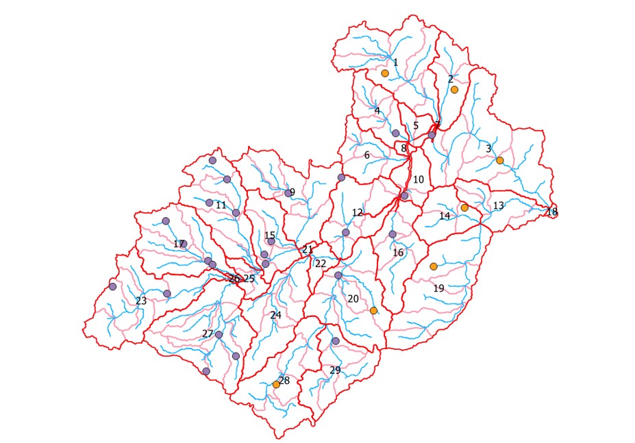 As promised, we will wrap this section on data preparation up by looking into
the spatial distribution of the meteorological stations. As indicated earlier, SWAT+ looks for each of the identified HRUs for the closest weather station. This can
lead to selecting a station that is located far away from the HRU and, thus, a misrepresentation of the meteorological conditions. This can be avoided by planting
virtual stations with empty time series (i.e. a value of -99) throughout the basin. By doing so, we force SWAT+ to simulate weather conditions in said particular spot.
The graph on the right illustrates this by showing existing (purple) and virtual (orange) stations in the Paute basin, to avoid selecting a station too far away.
As promised, we will wrap this section on data preparation up by looking into
the spatial distribution of the meteorological stations. As indicated earlier, SWAT+ looks for each of the identified HRUs for the closest weather station. This can
lead to selecting a station that is located far away from the HRU and, thus, a misrepresentation of the meteorological conditions. This can be avoided by planting
virtual stations with empty time series (i.e. a value of -99) throughout the basin. By doing so, we force SWAT+ to simulate weather conditions in said particular spot.
The graph on the right illustrates this by showing existing (purple) and virtual (orange) stations in the Paute basin, to avoid selecting a station too far away.
This section marks the end of the data preparation for model development, thus we can continue with the development of the actual hydrological model. More information related to this can be found on the page related to Model calibration.