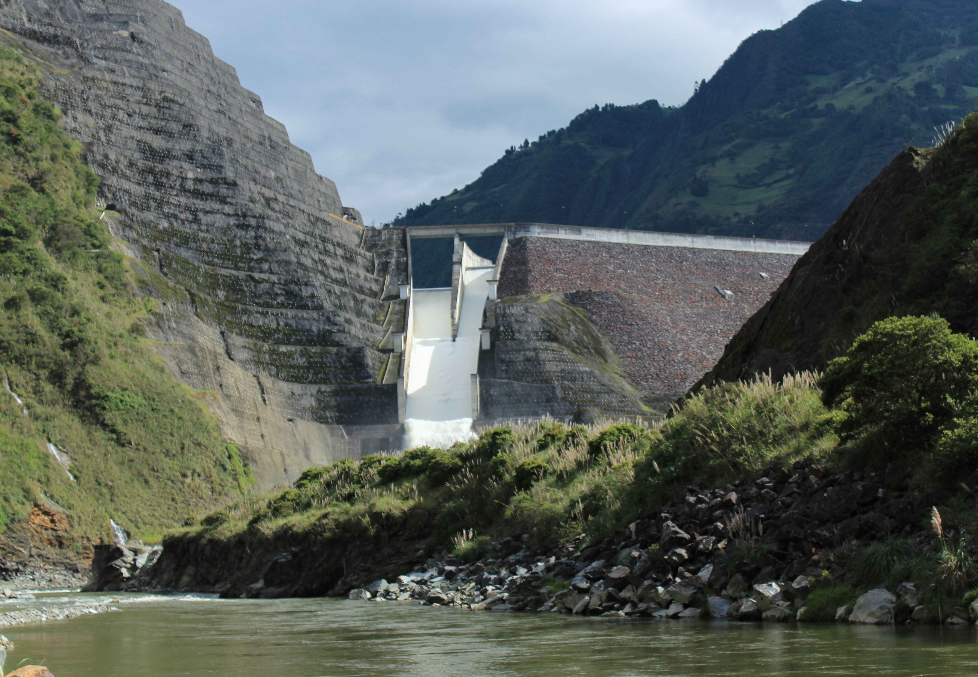
Within the HydroCORE project, eight field monitoring campaigns were conducted to gather information on the emissions of greenhouse gases in about 50 sites, distributed over two basins (Paute and Jubones) and two freshwater types (flowing and stagnant). At each location, a floating chamber was connected to the river bank (bigger rivers), to some stones in the river itself (smaller rivers and streams), or to the boat (reservoir sites). The chamber itself was made airtight with a single septum at the top for collecting samples and covered with aluminium foil for insulation. A general air sample at 1 meter above the water surface was collected to represent the reference or start situation. A second sample was collected from the floating chamber after 20 minutes, followed by a third sample after another 20 minutes (hence, 40 minutes in total). Each sample was equal to 20 mL, which was transferred to a 12 mL glass vial (prerinsed three times with Helium) and send to ETH Zürich for greenhouse gas analysis.

The obtained concentrations reported by the equipment reflect the composition of (1) the atmosphere (the reference sample) or (2) the composition of the air in the headspace of the floating chamber. Additional calculations are needed to transform these concentrations into fluxes, requiring both the headspace volume and the water surface within the chamber. A linear regression is performed for the greenhouse gas concentration in function of time, resulting in a value for the slope of the regression line. The associated R-squared value is used to identify valid observations for flux calculations, resulting in the exclusion of sample series for which the R-squared value does not exceed 0.5. Ultimately, the greenhouse gas emissions were calculated in mg/m²/d.

Some observations related to these gas emissions can be found below, which is an extension of the short description provided in the campaign-specific pages [link] and reports [link].

To start our exploration of the emitted greenhouse gas data, we look at the distribution of the calculated values and how they relate to each other. More specifically, the derived density plots show us that the three considered gases display overlapping ranges: carbon dioxide emissions cover the widest range and typically fall between -500 mg/m²/d and 800 mg/m²/d, while methane emissions range from 0 to 50 mg/m²/d and nitrous oxide levels range from 0 and 3 mg/m²/d. In other words, one can expect carbon dioxide emissions to be higher than methane levels, while nitrous oxide emissions constitute the smallest fraction. At the same time, the negative values that were obtained for the carbon dioxide emissions suggest that some sites can act as sinks rather than sources.

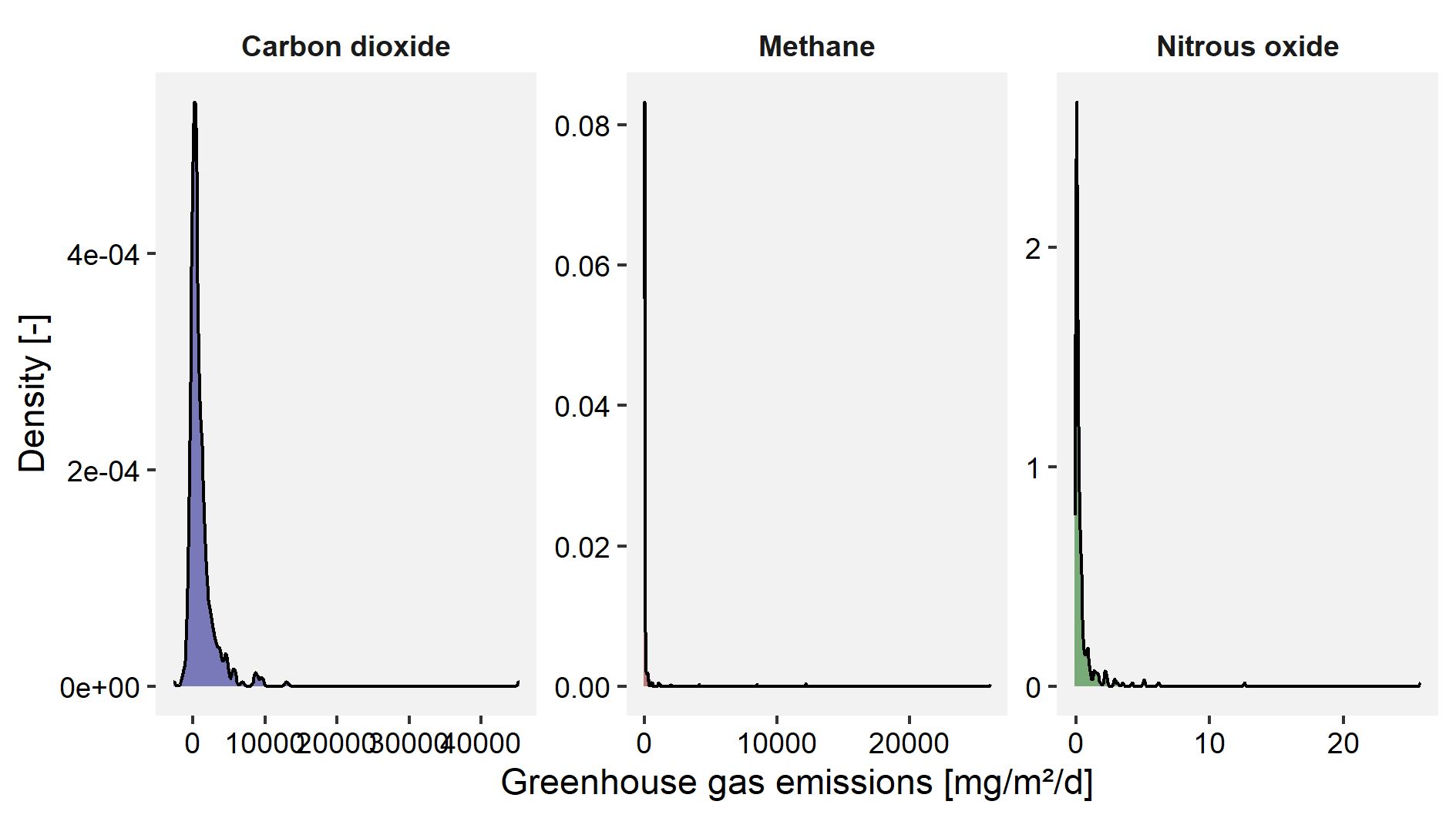
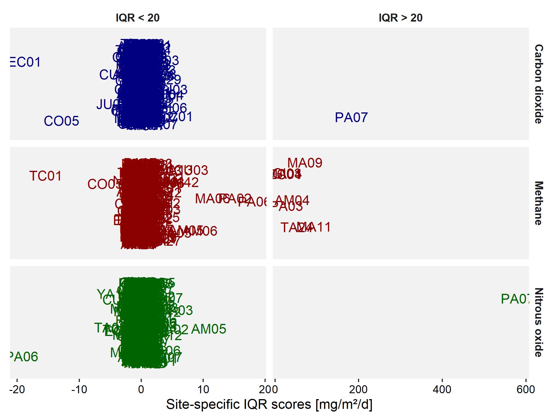
From the density plots, it can be observed that there might be some exceptionally high levels of emitted greenhouse gases present in our database. A deeper look into the presence of potential outliers can provide an answer to this. In order to be able to compare the analyses for all three greenhouse gases, a site-specific factor is calculated that represents the distance of a value from the median value in terms of the inter-quartile range (IQR). More specifically, a subset is derived from the main data set for each combination of sampling site and greenhouse gas, over all campaigns (hence, resulting in a subset of maximally 8 observations). Then, the median of this subset of greenhouse gas values is subtracted from the subset of individual greenhouse gas values, followed by a division by the IQR for the same subset of greenhouse gas values. The resulting distance factor directly gives an idea of how far each individual observation is removed from the sample- and gas-specific median value. For instance, a site with a distance factor of -2 is situated at twice the IQR from the median in the negative direction.

This analysis indicates that especially methane is characterised by a couple of values that are relatively high when compared to all values obtained at the same site over all campaigns, followed by nitrous oxide and carbon dioxide. Based on the tabular overview, it can be derived that methane emissions during the sixth campaign were relatively high in locations MA09 and TA24, when compared to the other campaigns in the same sites. Also site MA11 displayed a relatively high methane emissions during campaign 8, while site PA07 showed a relatively high emission level of both carbon dioxide and nitrous oxide during campaign 6. A cutoff point at a distance factor of 20 can be considered here to help identifying (and removing) potential outliers prior to further analyses.

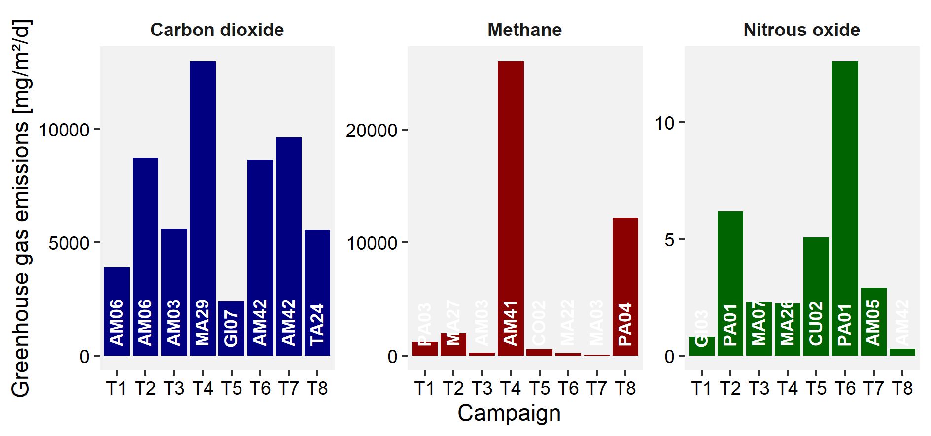
The abovementioned cutoff point at a distance factor of 20 results in the exclusion of some values for further analysis. More specifically, it supports the exclusion of 3 observations for carbon dioxide, 7 observations for methane, and 1 observation for nitrous oxide. Now that these more extreme values have been excluded, we can take a deeper look at the lowest and highest emission levels of greenhouse gases observed within each campaign. By doing so, it can be observed that both the lowest and the highest emissions for each of the greenhouse gases vary greatly among the different campaigns, with methane displaying the highest variability (being highest in campaigns 4 and 8, which were characterised by high water flows).

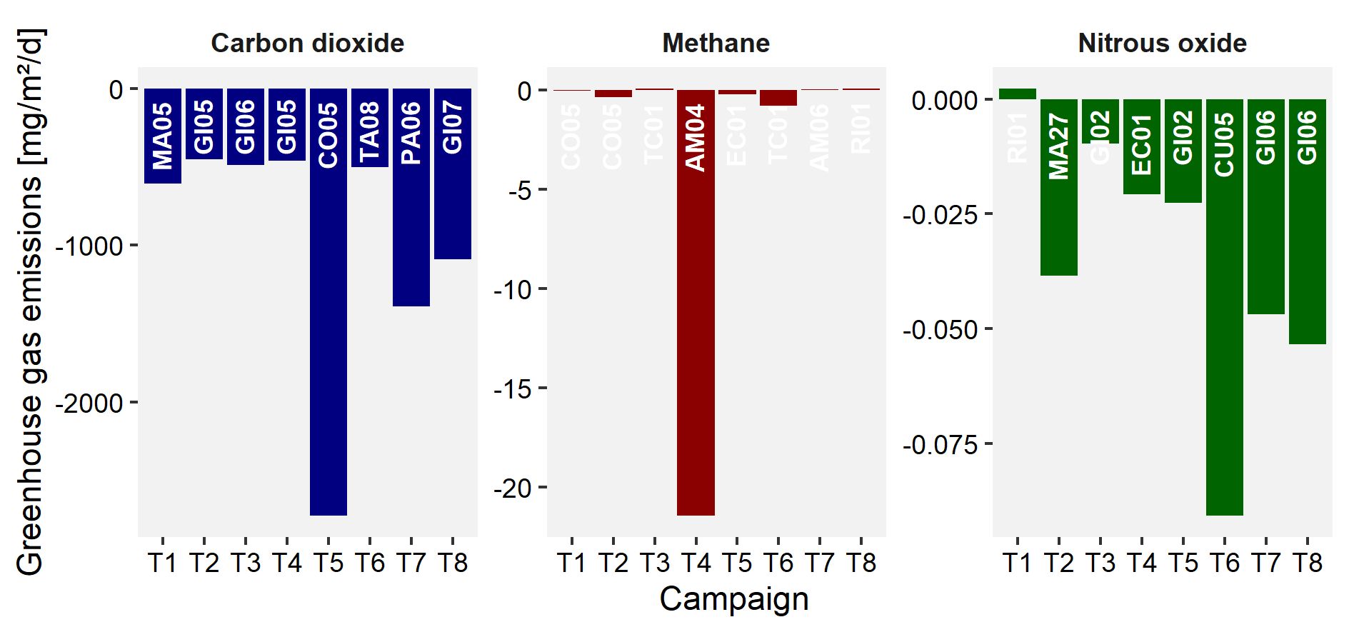
In contrast, nitrous oxide emissions showed to be highest in site PA01 during campaign 6, when an extreme drought was taking place. In addition, it is also remarkable that each of the considered gases can also be taken up instead of emitted to the atmosphere, as indicated by the (highly variable) negative values. When comparing these values, it is good to keep in mind that both sites AM03 and AM04 were heavily covered by water hyacinth whenever samples were collected.

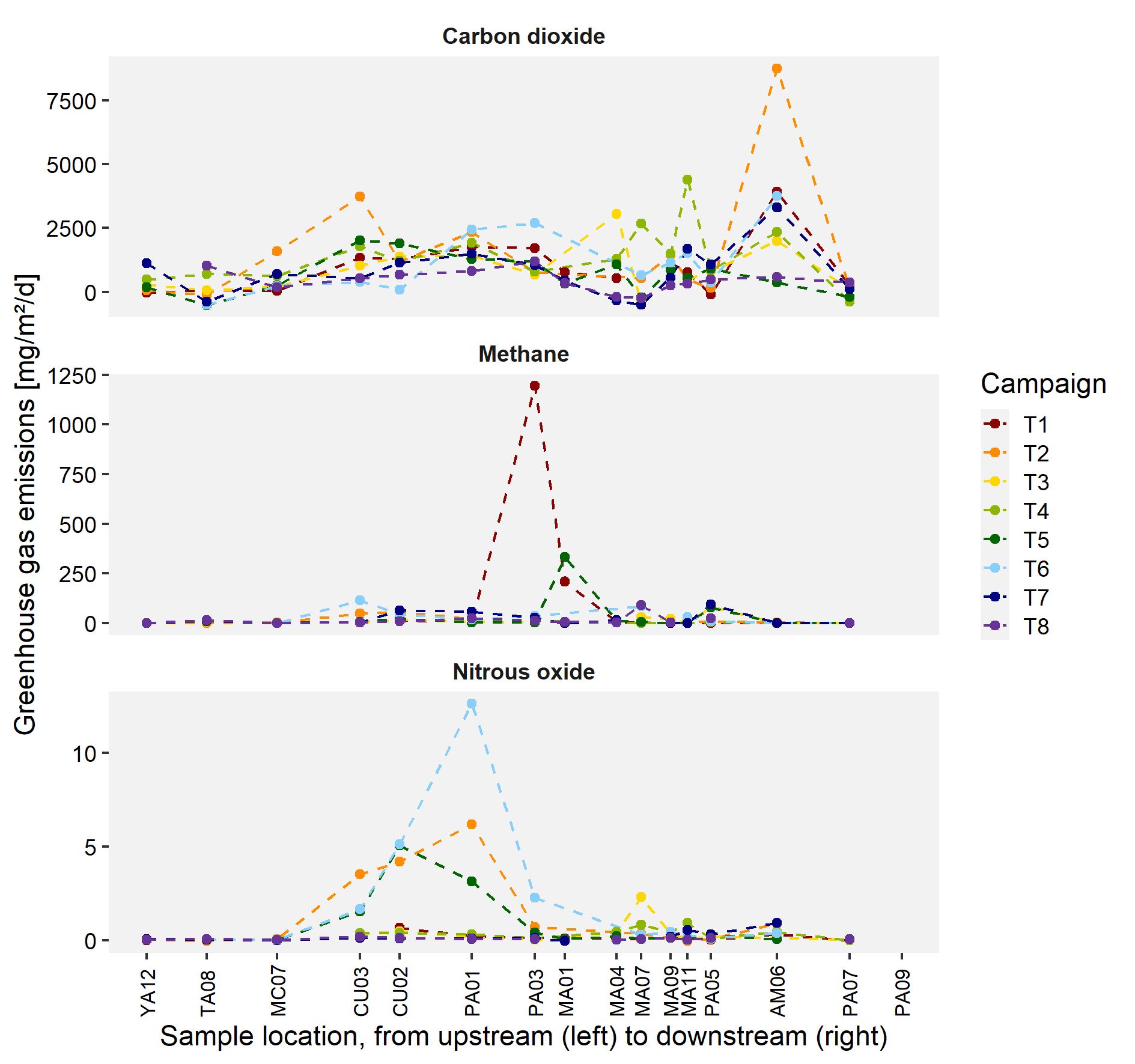
Aside from the temporal variability, we are also interested in the spatial variability and how greenhouse gas emissions change throughout the sampled river system. Via a subset of sampling locations, the spatial variability is displayed and shows an increase in carbon dioxide and nitrous oxide emissions downstream of the city of Cuenca during the drought campaigns (2 and 6), as well as in the upstream part of the Mazar reservoir (methane in MA01). Carbon dioxide emissions decrease slightly towards the downstream section of the Mazar reservoir, though seemingly increase again when present within the Amaluza reservoir. Over all, it can be said that nitrous oxide emissions increase due to the presence of the city of Cuenca, while also slightly increasing the emissions of carbon dioxide. Methane emissions seem to remain relatively stable throughout the system, though a single high value can mask more subtle changes.

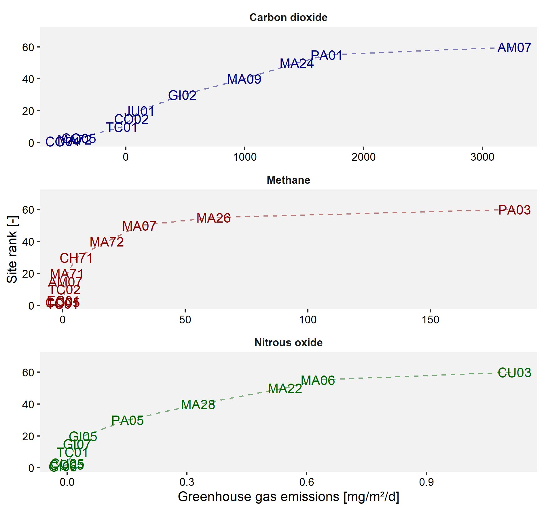
Lastly, all available data is compiled into a single average level of emitted greenhouse gases per site to identify those sites that are, on average, the sites with the highest and lowest levels of greenhouse gas emissions. From this, it is clear that several sites stand out and that no single site is characterised by the highest emissions of two or three of the considered greenhouse gases. The site AM07 (close to the dam of the Amaluza reservoir) displays the highest carbon dioxide emissions, while PA03 (right before the start of the Mazar reservoir) has the highest methane emissions and site CU03 (directly downstream of the city of Cuenca) shows the highest nitrous oxide emissions. It is noticeable that several sites within the Mazar reservoir are characterised by having emissions that are higher than the average emission levels, whereas the Collay part of this reservoir (codes 'CO') can often be found at the complete opposite side. It should be noted that the depiction has been simplified by having only a subset of all sites, though the top and bottom three sites for each greenhouse gas are always included.

From these observations, it is clear that there is a relatively high level of variability in the emission levels of the three considered greenhouse gases. The exceptionally high values can be ascribed to contaminated or badly rinsed gas vials, as well as to bad luck during sampling (e.g., an accidental ebullition event that was captured by the floating chamber), or to damage during transport. The generic approach to identify these potentially erroneous values allows for some data cleaning, though not all outliers might have been filtered out and a more in-depth approach to identify these is recommended prior to making strong statements. Yet, it also remains possible that these values correctly depict the actual situation at the time of sampling.

The remainder of the analysis shows that several sites support the uptake of the three greenhouse gases, though this quantity is highly variable in time. The maximum emission level of all three greenhouse gases are frequently observed in the reservoir sites (both Mazar and Amaluza) and complemented with other sites that experience some kind of human impact (e.g., the Cuenca river, the Giron system). It still remains to be seen how these levels are linked with the local biotic community and the dissolved levels of the considered greenhouse gases. More information on the latter can be found here.